Freeform curves 自由曲线

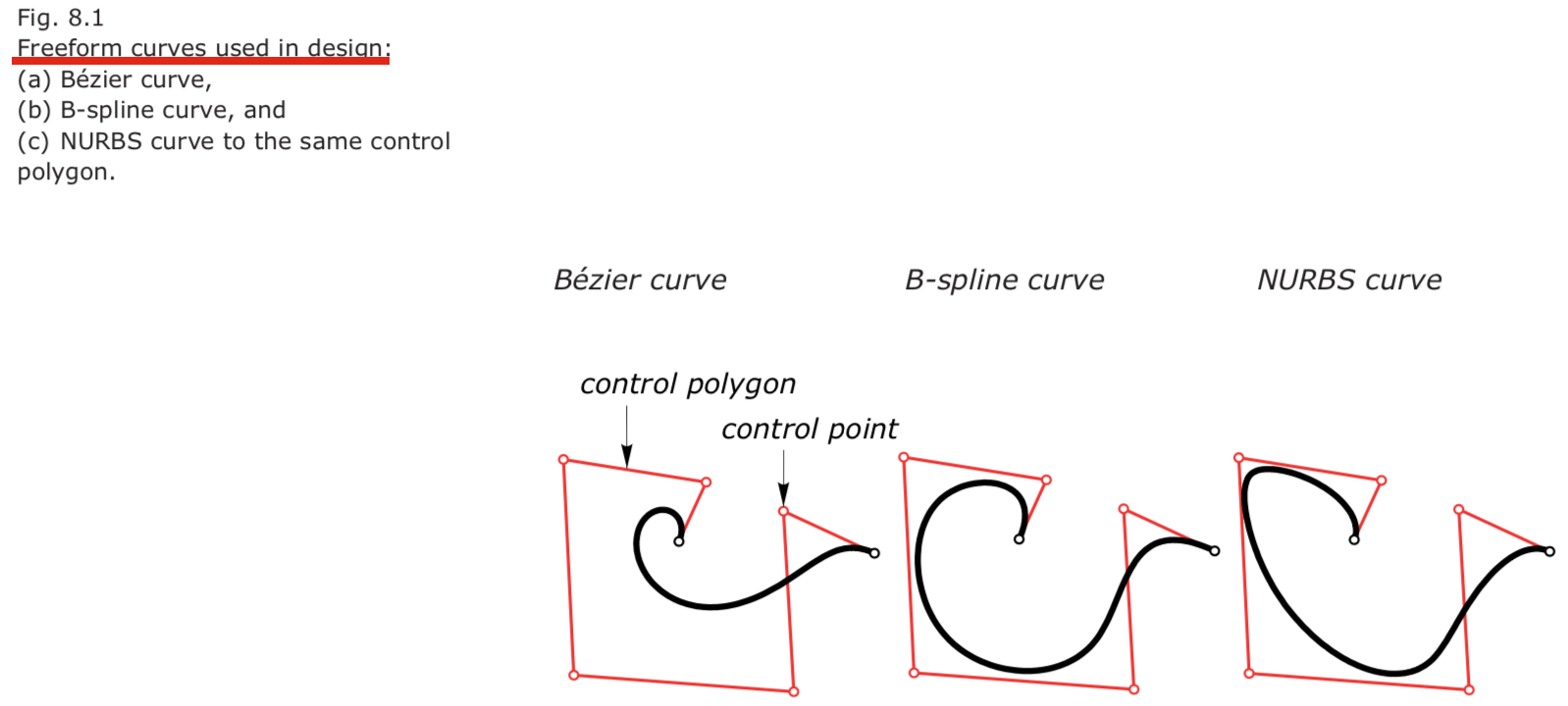
Bezier Curves

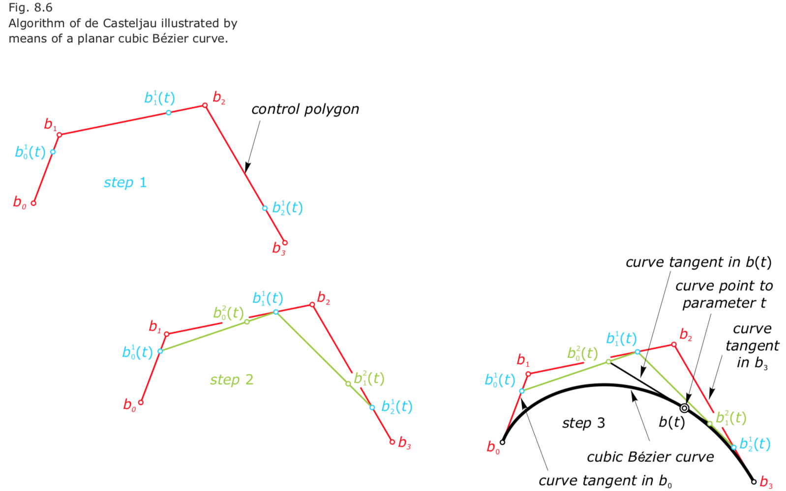
• To generate a point on a Bézier curve with $n$ control points, we have to perform $n – 1$ steps of the de Casteljau algorithm. $n$个控制顶点，$n-1$次曲线，需要$n-1$次算法

• 局限：
  
  1. A Bézier curve with a large number of control points becomes impractical for design. The degree of the curve increases and the curve shape resembles less the shape of the control polygon. \
  2. The control points have global control on the shape of the curve.

B-spline Curves

• The B stands for “basis.”
• We can also use the B as a mnemonic to remember that a B-spline curve consists of several Bézier curve segments.
• Defining a B-spline curve. A B-spline curve is defined by
  

  • $m + 1$ control points,
  • the degree $n,$ and
  • the knot vector.
  

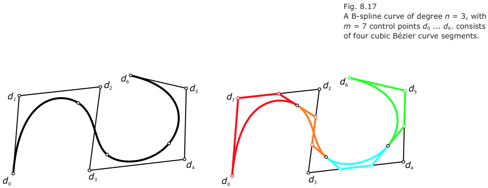
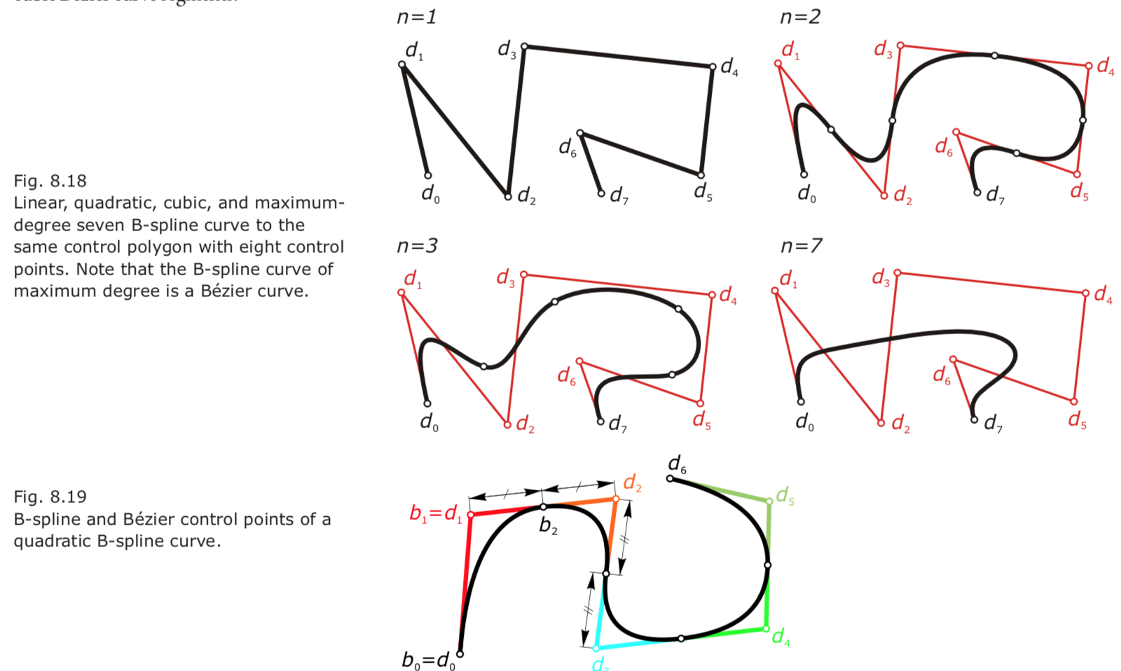
• B-spline curve of degree $n$ with $m + 1$ control points $d_0, d_1, … d_m$ consists of $m + 1 – n$ Bézier curve segments of degree $n$.
• The maximum degree achievable is $n = m$, for which the B-spline curve is actually a Bézier curve to the same control polygon.

• The human eye is able to detect kinks (because the curve tangents change abruptly) and curvature discontinuities (because the curvature changes abruptly). For cubic B-spline curves, we inherently achieve smooth tangents and smooth curvature at the knot points where the separate curve segments are joined.

• B-spline curves 缺点： With B-spline curves, we are not able to represent such simple curves as a circle, an ellipse, or a hyperbola.

NURBS Curves

• NURBS curves are B-spline curves with a nonuniform knot vector.

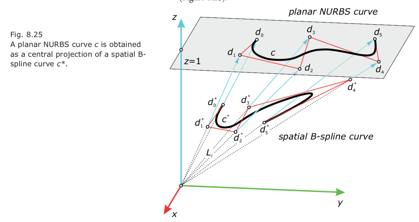
• Connection between B-spline curves and NURBS curves: a planar NURBS curve is a central projection of a spatial B-spline curve.
• In addition, a spatial NURBS curve is a central projection of B-spline curve lying in a 4D space.
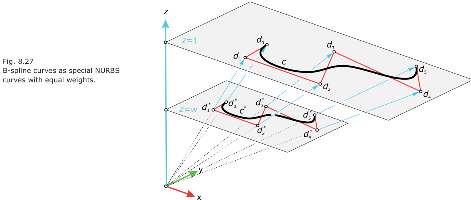
• A B-spline curve is a special NURBS curve wherein all weights are equal.

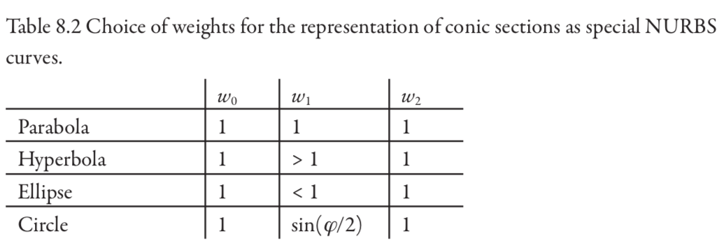
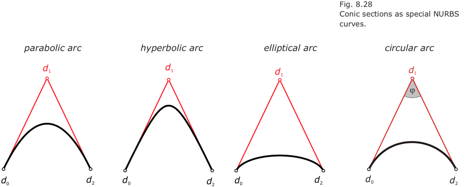
• Conic sections as special NURBS curves.

Subdivision curves 细分曲线

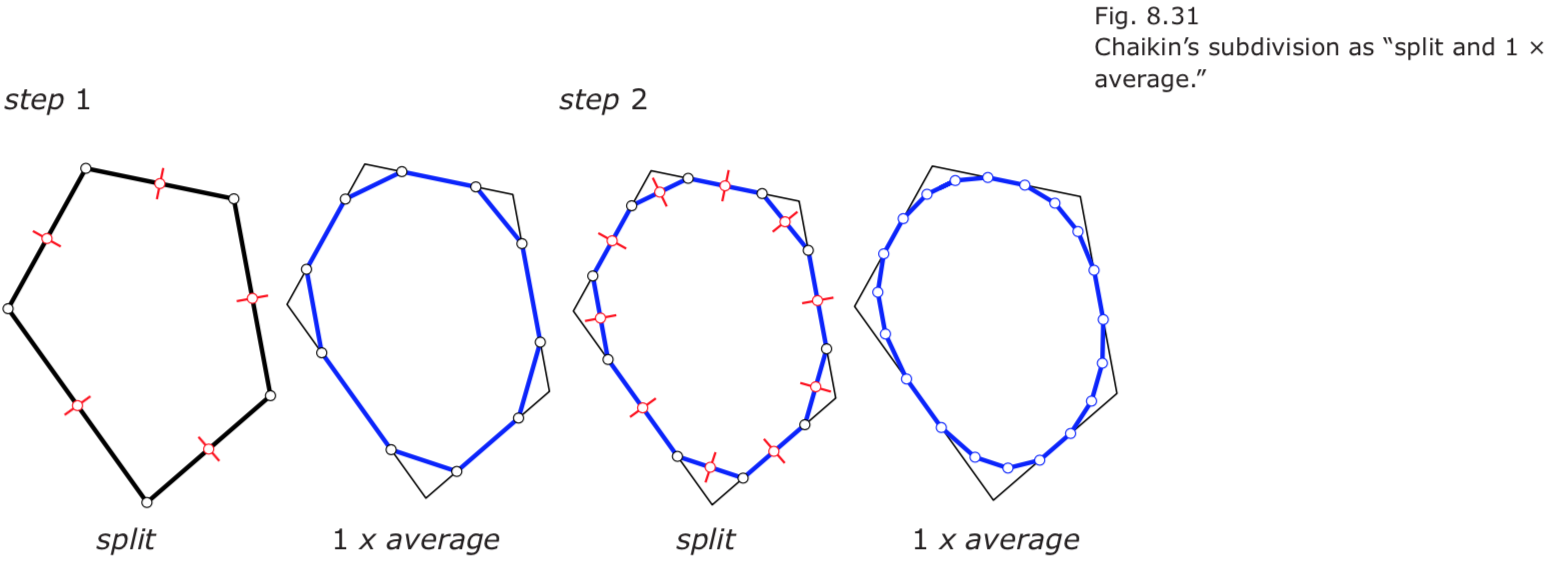
• Chaikin’s algorithm for the generation of quadratic B-splines.

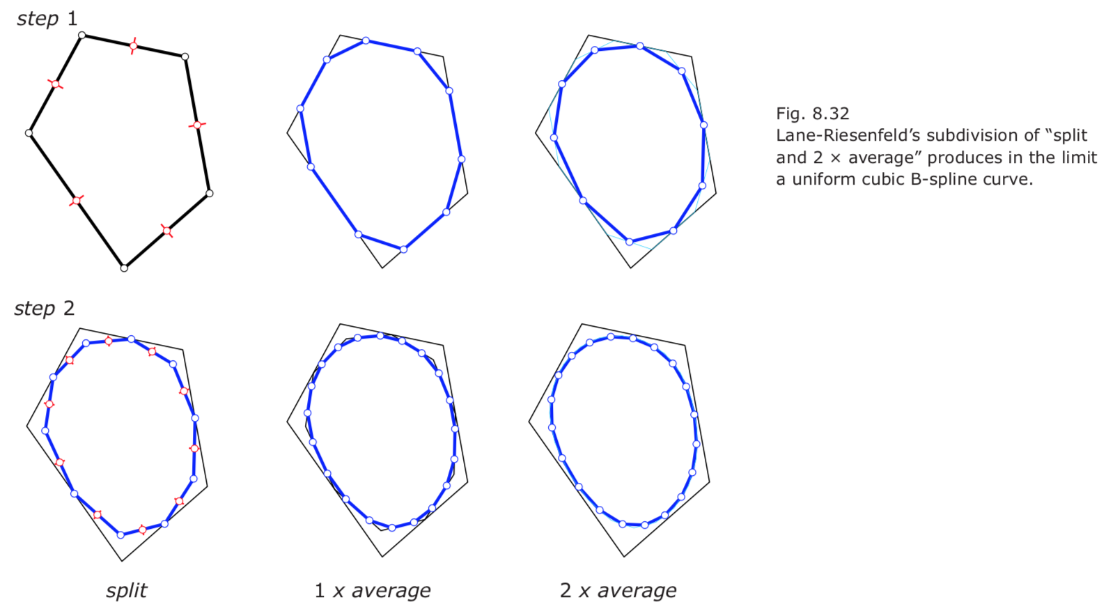
• The Lane-Riesenfeld algorithm is a generalization of Chaikin’s algorithm that produces in the limit a uniform B-spline curve of degree n.

• The four-point scheme of Dubuc. Formally, the new point is computed as

  $p_i^{new} = –1/16 p_{i-1} + 9/16 p_i + 9/16 p_{i+1} – 1/16 p_{i+2}.$

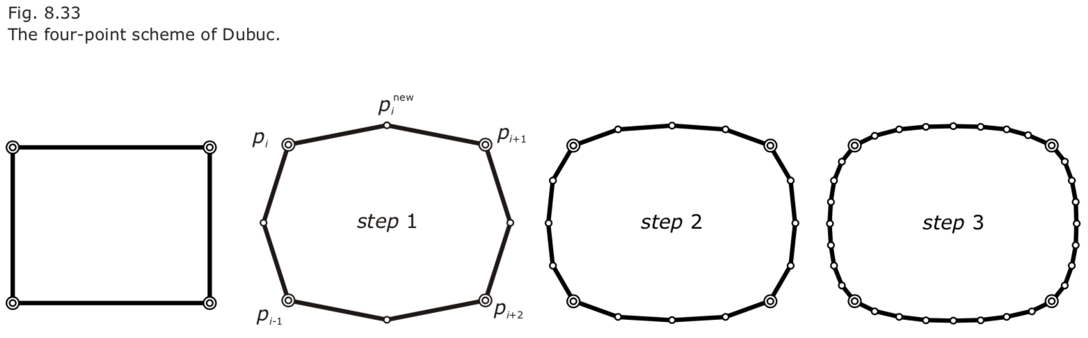
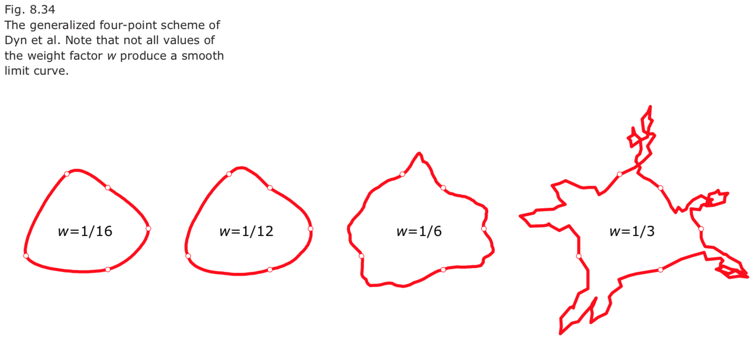
• One year later, Dyn et al. (1987) generalized the four-point scheme as follows.

  $p_i^{new} = –w∙p_{i-1} + (1/2 + w)∙p_i + (1/2 + w)∙p_{i+1} – w∙p_{i+2}.$

For w = 1/16 we have the original four-point scheme.